Books analysis using AI
tldr: Figuring out myself from books I read using all kinds of data analysis methods. Things does get interesting
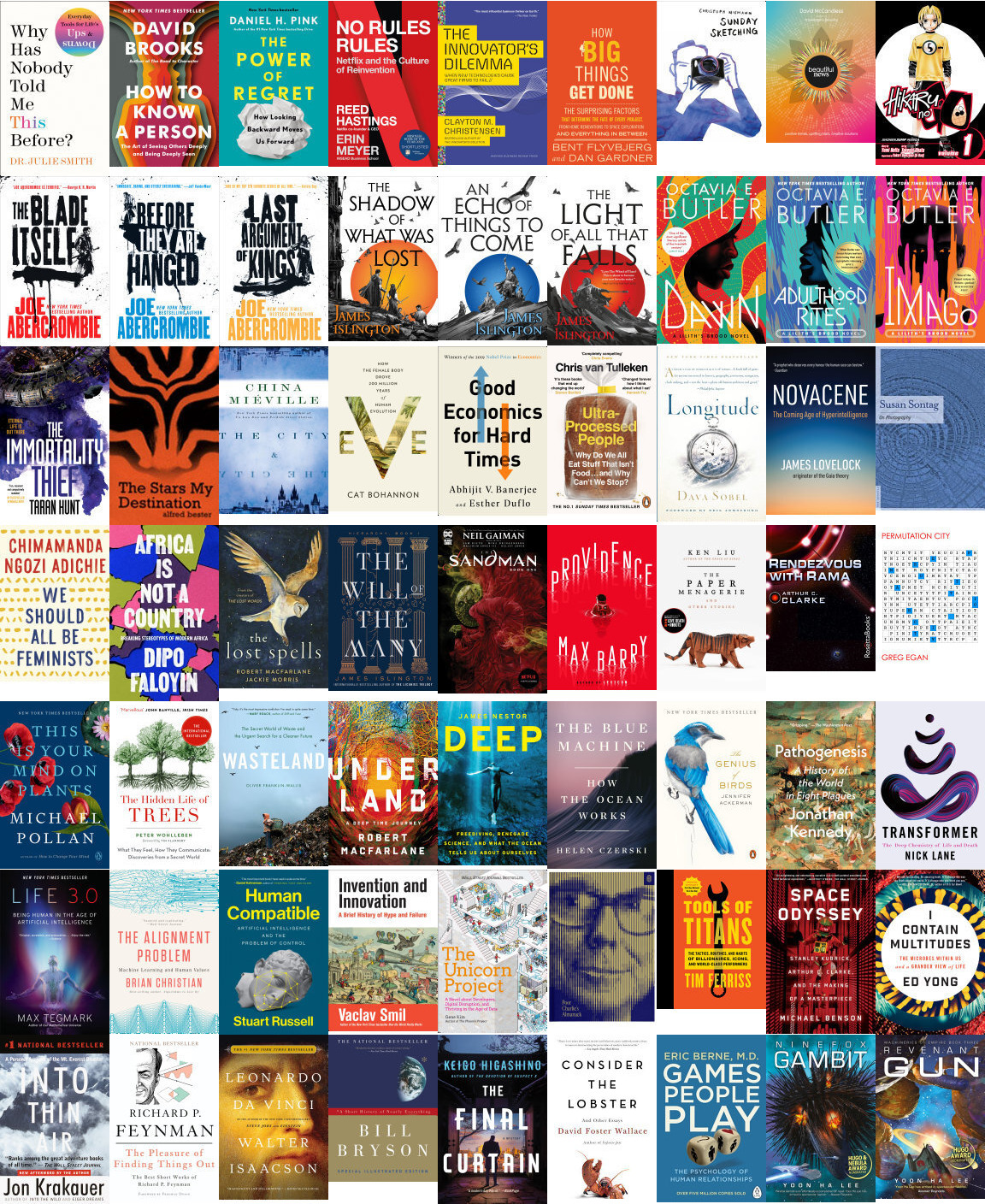
I always wanted to do this analysis, but the data of my shelf wasn't big enough before and since I paused reading for summer let's do this finally. We will start with 2024 read books so far, but will go onto my whole read bookshelf as things get interesting.
Note: This is still a high level napkin plan, but we will figure things out as we go. This is also a testbed for my upcoming two large scale free opensource AI projects for books. stay tuned 😉
part 1: data processing
# get covers from google books using book ids
import requests
import time
import random
with open("google_book_ids_2024", "r") as f:
    #file containing ids ordered as per genre and series
    gids = f.read().splitlines()
for i, gid in enumerate(gids):
    crawl_cover_url = f"https://books.google.com/books/content?id={gid}&printsec=frontcover&img=1&zoom=1"
    cover_image = requests.get(crawl_cover_url)
    i_str = str(i).zfill(3)
    with open(f"{i_str}_{gid}.jpg", "wb") as f:
        f.write(cover_image.content)
    antiblock = random.randint(1, 5)
    time.sleep(antiblock)
Now lets make a collage with imagemagick to see our covers
#!/bin/bash

files=($(ls *.jpg | sort))
magick -size 1000x1 xc:white collage_books_2024.jpg
for ((i=0; i<${#files[@]}; i+=9)); do
    # my preference of 9 for row, as i love trilogies and this fits best
    batch=(${files[@]:i:9})
    magick "${batch[@]}" +append row.jpg
    magick collage_books_2024.jpg row.jpg -append collage_books_2024.jpg
done
rm row.jpg
part 2: standard book covers analysis
Now, we start by getting all color pixels from all these book covers and try to see aggregate color pattern. We work with hsv image space since it's intuitive and do the colors plot radially in 2d by collapsing the value dimension and sticking with hue, saturation to denote. We will do k-means clustering to cluster points and plot according to levels for easy demarcation. I chose 8 here as a way to get 8 radial circles but seems the clusters are more than that, instead of doing elbow curve and selecting best cluster size, we will skip it for more interesting part in part 3. Let's go process those 3.179 million pixels now.
import numpy as np
import cv2
from sklearn.cluster import KMeans
import matplotlib.pyplot as plt
from mpl_toolkits.mplot3d import Axes3D

from collections import Counter
import os
import glob

dir_path = os.path.dirname(os.path.realpath(__file__))
image_paths = sorted(glob.glob(os.path.join(dir_path, "*.jpg")))
images = [cv2.imread(path) for path in image_paths]

np.random.seed(42)
histograms = []
total_pixels = 0
for img in images:
    img = cv2.cvtColor(img, cv2.COLOR_BGR2HSV)
    pixels = img.reshape(-1, 3)
    hist = Counter(map(tuple, pixels))
    histograms.append(hist)
    total_pixels += img.shape[0] * img.shape[1]
print('Total Pixels:', total_pixels)
combined_hist = sum(histograms, Counter())

pixels = np.array(list(combined_hist.keys()))
hue = pixels[:, 0] / 180.0 * 2 * np.pi  # Convert hue to range [0, 2*pi] and opencv hsv hue range is [0, 180]
original_pixels = pixels.copy()

pixels[:, 0] = np.cos(hue)
pixels = np.column_stack((pixels, np.sin(hue)))  # Adding sin(hue) as a new dimension to consider conical periodicity of hsv

weights = np.array([3*256, 1, 1, 3*256]) # more weight to hue as with human perception and scaling as per max value of all channels
weighted_pixels = pixels * weights
kmeans = KMeans(n_clusters=8, random_state=42) # 8 clusters chosen to represent 8 radial rings for planets in solar system
# did i just invent astrovisualization? :P
labels = kmeans.fit_predict(weighted_pixels)
# print('distortion:', kmeans.inertia_)

saturation = pixels[:, 1] / 255.0
cluster_sizes = np.bincount(labels)
sorted_cluster_indices = np.argsort(cluster_sizes)
label_mapping = np.zeros_like(sorted_cluster_indices)
label_mapping[sorted_cluster_indices] = np.arange(kmeans.n_clusters)
new_labels = label_mapping[labels]
normalized_new_labels = new_labels / (kmeans.n_clusters - 1)
saturation = saturation + normalized_new_labels
saturation = saturation - np.min(saturation)
normalized_saturation = saturation / np.ptp(saturation) #scaling to [0, 1]
x = normalized_saturation * np.cos(hue)
y = normalized_saturation * np.sin(hue)

fig = plt.figure(figsize=(10, 10))
for i in range(kmeans.n_clusters):
    cluster_indices = (labels == i)
    cluster_colors = original_pixels[cluster_indices]
    cluster_colors = cluster_colors.reshape(-1, 1, 3)
    cluster_colors = cv2.cvtColor(cluster_colors, cv2.COLOR_HSV2RGB)
    cluster_colors = cluster_colors.reshape(-1, 3) / 255.0 #scatter takes rgb in [0,1]
    plt.scatter(x[cluster_indices] , y[cluster_indices], c=cluster_colors, alpha=0.5, s = 10)

plt.title('HS(-V) plot with KMeans Clustering')
fig.savefig('books_hs_scatter_plot_.png')
Now let's create rorschach preliminary image from same data because why not and it's pride month.
original_x, original_y = x.copy(), y.copy()
y = y /2
x,y = y,x
rotated_x = y
rotated_y = x
mirrored_x = -rotated_y
mirrored_y = rotated_x

separation = 0.18
rotated_y += separation / 2
mirrored_x -= separation / 2

fig = plt.figure(figsize=(10, 10))
for i in range(kmeans.n_clusters):
    cluster_indices = (labels == i)
    cluster_colors = original_pixels[cluster_indices]
    cluster_colors = cluster_colors.reshape(-1, 1, 3)
    cluster_colors = cv2.cvtColor(cluster_colors, cv2.COLOR_HSV2RGB)
    cluster_colors = cluster_colors.reshape(-1, 3) / 255.0

    plt.scatter(x[cluster_indices], y[cluster_indices], c=cluster_colors, alpha=0.7, s=8)
    plt.scatter(mirrored_x[cluster_indices], mirrored_y[cluster_indices], c=cluster_colors, alpha=0.7, s=8)

plt.ylim(-1, 1)
plt.xlim(-.5, .5)
plt.grid(False)
plt.axis('off')
fig.savefig('books_rorschach_plot_.png')
The 2d plot above collapsed the color count into 1d. We also want to look at how popular a particular color is, so let's create a density height map plot. I love those population density plots of cities.
# 3d density
x,y = original_x, original_y
xy = np.vstack([x, y]).T
xy_unique, counts = np.unique(xy, axis=0, return_counts=True)
xy_unique, indices = np.unique(xy, return_inverse=True, axis=0)
unique_colors, color_indices = np.unique(original_pixels.reshape(-1, 3), axis=0, return_inverse=True)
cluster_colors = np.zeros((len(xy_unique), 3), dtype=np.uint8)
for i, index in enumerate(indices):
    cluster_colors[index] = original_pixels[i]
cluster_colors = cluster_colors.reshape(-1, 1, 3)
cluster_colors = cv2.cvtColor(cluster_colors, cv2.COLOR_HSV2RGB)
cluster_colors = cluster_colors.reshape(-1, 3) / 255.0
fig_3d = plt.figure(figsize=(10, 10))
ax = fig_3d.add_subplot(111, projection='3d')
x_unique = xy_unique[:, 0]
y_unique = xy_unique[:, 1]
z_bottom = np.zeros_like(counts)
dx = dy = 0.01
dz = counts
ax.bar3d(x_unique, y_unique, z_bottom, dx, dy, dz, color=cluster_colors, alpha=0.8)
ax.xaxis.set_pane_color((1.0, 1.0, 1.0, 0.0))
ax.yaxis.set_pane_color((1.0, 1.0, 1.0, 0.0))
ax.zaxis.set_pane_color((1.0, 1.0, 1.0, 0.0))
ax.set_xlabel('hue cos')
ax.set_ylabel('hue sin')
ax.set_xticks([-1, 0, 1])
ax.set_yticks([-1, 0, 1])
ax.set_zticks([])
ax.grid(False)
ax.view_init(elev=25, azim=-47)
plt.title('HS color density plot')
fig_3d.savefig('books_hs_density_plot_3d_.png')
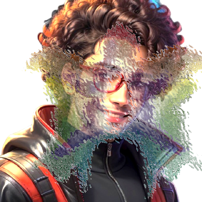
We will do basic photo affects for final filter and hand smudge to make the rorschach my own. Shoutout to my fav photopea
Well, well, well. So how does my data look like? let's make the collage, already ordered via filenames.
find . -type f | grep '^[0-9]' | xargs -I {} sh -c 'convert "{}" -resize 720x720! miff:-' | montage -geometry +0+0 -tile 4x4 miff:- books_part1_collage.jpg
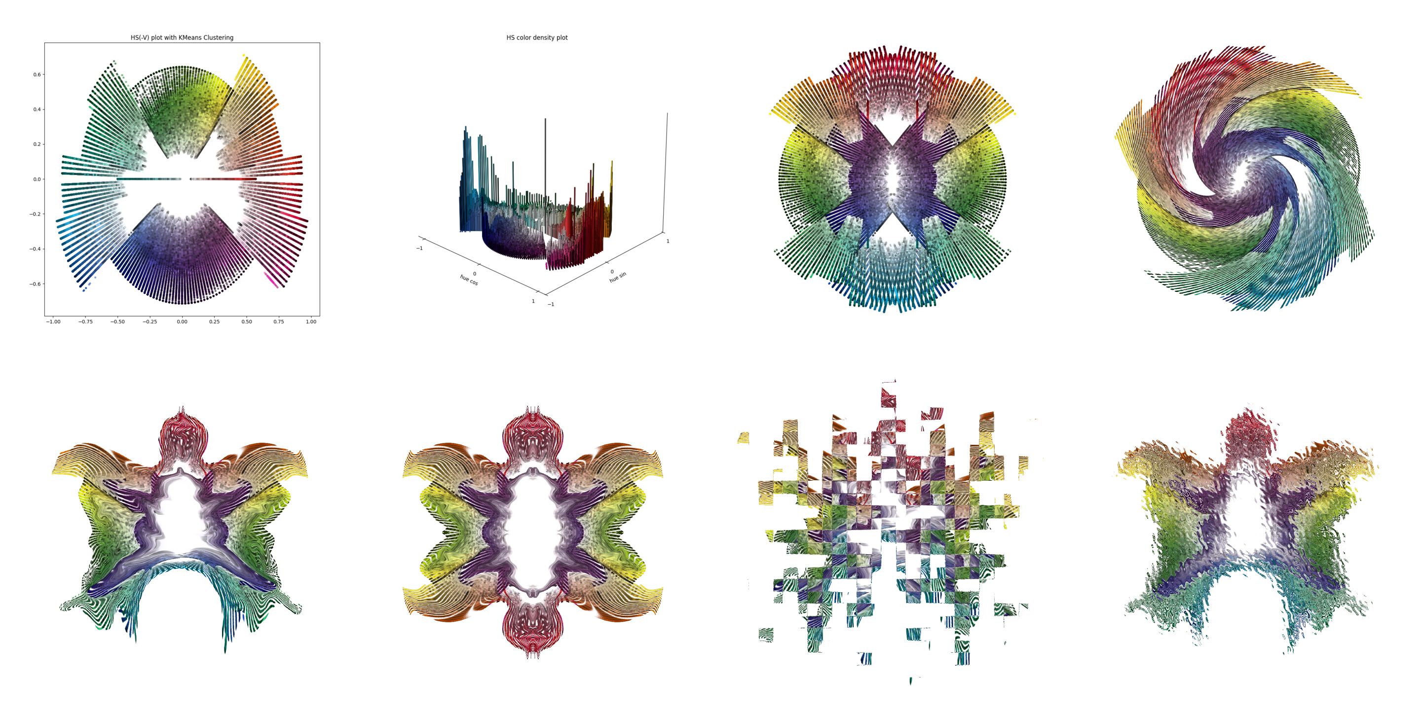
The seventh image was inspired from Rashid rana's War within artwork I saw at knma last month.
Now, let's combine pfp with filter.
convert pfp.jpg -modulate 88 -level 0%,70% \( filter.png -resize 140% -geometry +60+40 \) -gravity center -compose blend -define compose:args=65 -composite pfp_with_filter.png
Now we have to understand that context matters a lot in data.
Even if we didn't know the context, we were instructed to remember that context existed. Everyone on earth, they'd tell us, was carrying around an unseen history, and that alone deserved some tolerance. – Michelle Obama, Becoming
And aggregating entire color set as above did make things easy, but without the context it's missing a lot. I recently read art research on how our saccadic eye movements with right colors spatially connected can make Piet Mondrian paintings superior sub concsiously. So, we need to dig deeper in next part. stay tuned!
part 3: more color playing
- clustering the books based on color similarity and do standard network analysis and Graph Neural Networks.
- font size and textual placement data patterns on covers
- lets now do a color transfer between book covers based on similarity of their descriptions such that color palette intuitively shows similarity graph
part 4: book description analysis
- get description from google books using book ids
- We will do word clouds, topic modelling with latent dirchlet allocations and hierarchical dirichlet process, genre analysis, sentiment analysis and moods possible with read books using LLMs. Stay tuned!
part 5: more nifty visualizations and insights
- radial dendrograms, heatmaps and ...
part 6: generative imagery
- segment the covers and create kandinsky themed artwork with popular motifs
- using description of all books to generate a succint new master image, supposedly what ai brain imagines from its standpoint from all the books with their color transfer
final questions:
- is there significant correlation between color palette and genre of books?
- do we notice a temporal trend in the color palettes used in book covers? ofc some genres could have surged up at different timelines and I am biased on certain genres from certain years and I am selecting one color variation out of probably dozens of cover variants of that book, but still we can locate some patterns I hope
- Also check this interesting romance cover analysis by Alice liang in pudding —-